
Optical Computing GPU: Handing the Matrix to Light
From the von Neumann bottleneck to the latency, throughput, energy efficiency, precision and temperature control of a photonic tensor core, and what a hybrid graphics card of 2400 would look like
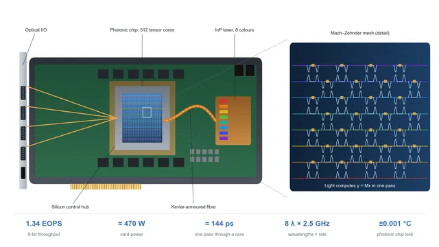
The HEO-GPU of 2400: a silicon control hub around a photonic tensor chip, fed by eight laser colours and held to a millikelvin.
The digital twins of 2400 (see how much data that world produces) recompute the lighting, materials and machine reasoning of the physical world every second. Break those workloads down and most of the computing goes into one operation: matrix multiplication. A 21st-century GPU uses tens of billions of transistors to perform multiply-accumulate operations one clock tick at a time, and pays for it at the power wall and the memory wall.
Light is naturally good at this. In a linear medium, light waves add by amplitude. Send a beam through a set of interferometers and the multiplications and additions happen while the light travels. Light also has weaknesses that cannot be engineered away: it cannot be made as small as a transistor, it is poor at nonlinear operations, and it is an analogue quantity. The graphics card of 2400 in The Digital Revolution is the result of dividing the work between these two carriers. This article starts from the von Neumann bottleneck and works out the latency, throughput, energy efficiency, precision and temperature control of a photonic tensor core, and what that hybrid card would look like.
Method: three levels of evidence
- Known physics (cannot be violated): superposition and interference of light in linear media, the unitary transformation of a Mach–Zehnder interferometer (MZI), the diffraction limit, photon shot noise, the thermo-optic effect in silicon, and the complexity of matrix operations.
- Existing experiments and theory (taken as the starting point): Reck and Clements meshes can realise any unitary matrix; the 2017 demonstration of an MZI optical neural network; co-packaged silicon photonics with external indium phosphide (InP) lasers; the published specifications of the RTX 4090 and RTX 5090.
- Engineering extrapolation (setting): high-speed DACs and ADCs at about 10 fJ per conversion, compact electro-optic MZIs of about 20 μm × 5 μm whose phase is held without power, 2.5 GHz modulation, and 512 tensor cores of 256×256 per card. These are marked setting in the text.
Numbers are labelled as measurement, assumption, calculation or setting. They are order-of-magnitude estimates for a fictional device, not a product specification.
The main findings
The "O(1)" of optical computing is about clock cycles, not distance. A matrix–vector product is done in one pass of light with no clock: about 144 ps through a 10 mm tensor core. The path still grows in proportion to N, at about 0.28 ps per column, and the number of devices grows as N². Matrices larger than the core must be cut into tiles.
The HEO-GPU of 2400 reaches about 1.34 EOPS at 8-bit precision for about 470 W. That is 512 tensor cores of 256×256 with 8 wavelength channels. Throughput is about 2,000 times an RTX 4090 and 1,600 times an RTX 5090; energy efficiency is about 2,800 TOPS/W, roughly 1,900 times either card.
The floor on energy is shot noise. At 8-bit precision each output needs at least about 66,000 photons.
The precision ceiling is about 8 bits. AI inference and light-transport solving can go to light; FP32, FP64 and branching logic stay with electronics. Electrons run the logic, light runs the matrices.
The film's temperature requirement of 25.000 ± 0.001 °C is the right order of magnitude. Temperature differences across one tensor core must stay below about 3 mK.
Table 1. Design baseline
| Parameter | Value | Basis |
|---|---|---|
| Photonic tensor core | 256×256 general matrix as $U\Sigma V^{\dagger}$: two Clements meshes of 32,640 MZIs plus 256 attenuators, 65,536 MZI-sized cells in total | Theory + setting |
| Cores per card, M | 512 (about 3.4×10⁷ MZIs, about 3,400 mm² of photonic chip) | Setting; area calculated |
| Modulation rate, f | 2.5 GHz | Setting |
| Wavelength channels, W | 8 (limited by phase dispersion) | Calculation |
| Operating wavelength | 1550 nm (photon energy 0.80 eV) | Measurement |
| Effective precision | 8 bits | Calculation (shot noise + temperature) |
| Conversion energy | About 10 fJ per DAC or ADC conversion | Setting |
| Temperature control | 25.000 ± 0.001 °C; differences within a core < 3 mK | Calculation |
| Comparison cards | RTX 4090: FP32 82.6 TFLOPS, FP8 dense about 660 TOPS, 450 W. RTX 5090: FP32 about 105 TFLOPS, FP8 dense about 838 TOPS, 575 W | Published specifications |
1. Matrices dominate the computing bill
A modern computer separates computing from storage: the processor calculates, the memory stores, and a bus carries data between them. Moving the data often costs more energy than the arithmetic. This is the von Neumann bottleneck, also called the memory wall. The ways out proposed in the 21st century each have their strengths:
Table 2. Division of labour among non-von Neumann architectures
| Approach | Method | Strength | Role in 2400 (setting) |
|---|---|---|---|
| In-memory computing | Multiply-accumulate inside the memory array | Removes data movement | Built into the lowest level of most chips |
| Neuromorphic computing | Spiking neurons and synaptic devices | Low-power, event-driven | Edge sensing |
| Quantum computing | Superposition and entanglement | Materials simulation, factoring, search | Coprocessor |
| Optical computing | Matrix multiply-accumulate by interference | Large-scale linear algebra | Tensor coprocessor (this article) |
The core of both AI inference and graphics rendering is linear. Each layer of a neural network is a matrix–vector product, and global illumination is a system of linear equations. Taking this part of the load away from electronics is what optical computing is for. The companion article on reversible computing places this tensor coprocessor alongside the other parts of a 2400 computer.
2. How light multiplies: the Mach–Zehnder interferometer
An MZI consists of two beam splitters and two phase shifters. Light enters by two ports, the two paths interfere at the second beam splitter, and each output amplitude is a linear combination of the input amplitudes:
Here θ is the internal phase shift and φ the external one (a global phase is dropped). This is a 2×2 unitary matrix: it conserves energy and only redistributes it between the two outputs.
Arrange N(N−1)/2 MZIs in a triangle (Reck, 1994) or a rectangle (Clements, 2016) and the mesh can realise any N×N unitary matrix. A general matrix is first split by singular value decomposition into two unitary matrices and a column of attenuators:
One 256×256 unitary mesh needs 256×255/2 = 32,640 MZIs. A general 256×256 weight matrix therefore needs two such meshes and 256 attenuators in series, 65,536 cells in all, equal to N². In this article a tensor core means this complete $U\Sigma V^{\dagger}$ unit. The weights are written into the phases of the phase shifters, the input vector into the amplitudes of the light, and photodetectors at the outputs read the result. In 2017 an MIT chip with 56 MZIs ran a vowel-recognition neural network this way (Shen et al.). The multiplication happens in the interference and the addition happens where the paths merge; neither needs a clock.
The next question is what the "O(1)" claimed for optical computing actually means.
3. What O(1) really means: one pass, no clock
The group velocity of light in a silicon waveguide is set by the group index, $n_g\approx4.2$, which gives about 7.1×10⁷ m/s, a little below the "order of 10⁸ m/s" quoted in the original concept. The latency of one operation is the time light takes to cross the mesh:
A Clements mesh is N columns deep. With 20 μm MZIs (setting), one 256-column mesh is 5.1 mm long and takes about 72 ps to cross; a full tensor core, with two meshes and the attenuator column, is 513 columns or about 10.3 mm, and takes about 144 ps. So the latency is not strictly independent of N: it grows in proportion to N, at about 0.28 ps per column. What does not appear is a clock. The whole product is formed in one pass, while the number of devices grows as N²:
Table 3. Complexity of matrix operations
| Operation | Electronics (operations) | Optical mesh (devices) | Optical mesh (time) |
|---|---|---|---|
| N×N matrix × vector | O(N²) | O(N²) MZIs | One pass; path length O(N) at about 0.28 ps per column |
| N×N matrix × matrix | O(N³); Strassen $O(N^{2.81})$; best theoretical bound $O(N^{2.371})$ | O(N²) | O(N) passes: feed one column at a time |
| K×K matrix × vector, K > N | O(K²) | O(N²) | O((K/N)²) passes: tiling |
The original concept said GPU matrix multiplication costs "at least O(N²) or $O(N^{2.37})$". That needs correcting. The dense matrix multiplication a GPU actually performs takes O(N³) multiply-accumulates. $O(N^{2.371})$ is a bound reached by theoretical algorithms whose constant factors are far too large to be used in practice. Optical computing turns O(N²) operations into O(N²) devices: it trades area for time. A matrix that does not fit on the chip must be cut into tiles, and the partial results from different tiles are summed back in the electronic domain.
A latency of a hundred-odd picoseconds does not mean the chip behaves like a clock running at several GHz. Throughput is set by two other quantities.
4. Throughput: from picoseconds to EOPS
A mesh can be pipelined: the next vector enters while the previous one is still inside. How many vectors per second can be sent in is set by the rate f of the modulators and detectors. The same mesh can also carry W wavelengths at once, each with its own vector. The equivalent operation rate of one card is:
The factor 2 counts one multiply-accumulate as two operations. With the setting values M = 512, N = 256, f = 2.5 GHz and W = 8:
The original concept imagined "dozens of wavelengths computing at once". But the phase of an MZI depends on wavelength. A phase is proportional to 1/λ, so a channel spacing of 0.8 nm changes it by a fraction of about 5×10⁻⁴, or about 3.2 mrad on a full 2π. Light in a silicon wire waveguide is also dispersive: the phase changes faster with wavelength than 1/λ alone, by roughly the ratio of group index to effective index, about 1.7. That makes each channel step cost about 5.6 mrad. Eight-bit precision allows a phase error of about 2π/256 ≈ 25 mrad, so with the phases set for the centre wavelength, about four channels fit on either side. W = 8 is therefore the setting value. Wavelength multiplexing is a real source of parallelism, but dispersion holds it to a handful of channels, not dozens.
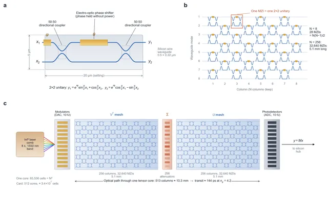
Figure 1. How a photonic tensor core is built. a, One electro-optic MZI (setting dimensions 20 μm × 5 μm): two 50:50 couplers and phase shifters θ and φ. b, A Clements mesh, shown for N = 8: N(N−1)/2 = 28 MZIs in N columns, so every path crosses the same number of devices. c, A general-matrix tensor core: V† mesh, attenuator column Σ and U mesh in series, about 10.3 mm long for N = 256, fed by modulators and read by photodetectors.
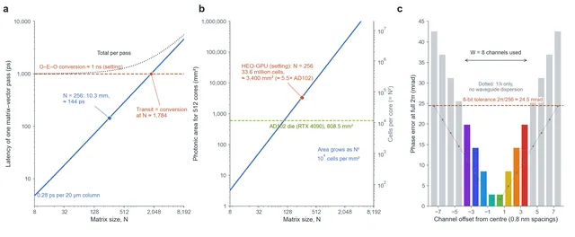
Figure 2. Scaling of a photonic mesh. a, Latency of one matrix–vector product against matrix size N: light transit through a tensor core grows linearly but stays below the 1 ns optical–electrical–optical conversion until N exceeds about 1,800. b, Devices per core (N²) and photonic area per card (512 cores at 10⁴ MZIs per mm²), compared with the AD102 die. c, Phase error of each wavelength channel relative to the centre, including waveguide dispersion, against the 8-bit tolerance of 2π/256.
5. The floor on energy: shot noise
Light is not a continuous fluid; it arrives as photons. When a detector counts n photons, the count fluctuates by about √n. To distinguish $2^B$ levels, the signal-to-noise ratio must reach $2^B$:
At 8 bits each output needs at least 65,536 photons. A photon at 1550 nm carries 1.28×10⁻¹⁹ J, so each output needs about 8.4×10⁻¹⁵ J. One output sums N = 256 multiply-accumulates, so the photon floor per MAC is about 3.3×10⁻¹⁷ J, or 256 photons per multiplication. Then add the insertion loss of the core (6 dB, a factor of about 4, setting, about 0.01 dB per cell), a laser wall-plug efficiency of 40% (setting), and the input and output conversions (10 fJ each, shared over N multiply-accumulates):
Table 4. Energy budget of one multiply-accumulate
| Item | Energy (J/MAC) | Notes |
|---|---|---|
| Photon shot-noise floor | 3.3×10⁻¹⁷ | 8 bits, N = 256 |
| Including loss and laser efficiency | 3.3×10⁻¹⁶ | ×4 loss, ÷0.4 wall-plug efficiency |
| DAC + ADC | 7.8×10⁻¹⁷ | 2 × 10 fJ ÷ 256 (setting) |
| Total | 4.05×10⁻¹⁶ | Photonic part: about 4,900 TOPS/W |
The card performs 6.7×10¹⁷ multiply-accumulates per second, so the photonic part draws about 270 W. With about 200 W for the silicon control hub, the whole card draws about 470 W, in the same class as today's flagship graphics cards:
Table 5. Comparison with the RTX 4090 and RTX 5090 (8-bit-class operations)
| Metric | RTX 4090 | RTX 5090 | HEO-GPU (setting) |
|---|---|---|---|
| 8-bit-class throughput | About 660 TOPS (FP8 dense) | About 838 TOPS (FP8 dense) | About 1.34 EOPS |
| Card power | 450 W | 575 W | About 470 W |
| Efficiency | About 1.5 TOPS/W | About 1.5 TOPS/W | About 2,800 TOPS/W |
| Throughput relative to 4090 | 1 | 1.3 | About 2,000 (1,600 relative to the 5090) |
| Efficiency relative to 4090 | 1 | 1 | About 1,900 |
The 5090 FP8 dense value is derived from NVIDIA's 3,352 AI TOPS, which is quoted for FP4 with sparsity. GPU figures are peak dense tensor throughput.
This comparison is for 8-bit-class tensor operations, not FP32. The efficiency gain of about 1,900 sits at the lower end of the original concept's "1,000 to 10,000 times". The throughput gain of about 2,000 is far above the concept's "more than a hundred times", and it comes from N² parallelism and wavelength multiplexing, not from a faster clock.
Shot noise sets a floor on energy, and it also draws a line for precision.
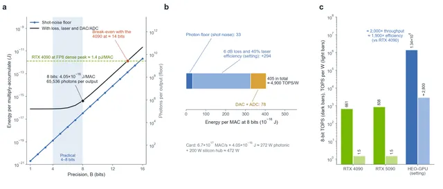
Figure 3. Energy and precision. a, Minimum photons per output and the photon-limited energy per MAC against precision B, for N = 256 at 1550 nm; each extra bit costs four times the light, and the total reaches the RTX 4090's energy per MAC at about 14 bits. b, Energy budget per MAC at 8 bits (Table 4). c, Throughput and energy efficiency of the RTX 4090, RTX 5090 and the HEO-GPU (setting) on logarithmic axes.
6. The precision ceiling and nonlinearity: why light specialises
Raising precision from 8 to 16 bits multiplies the photon count by 2¹⁶ = 65,536, which wipes out the entire efficiency advantage. Add fabrication error, thermal drift and laser power noise, and the practical precision of an optical mesh stops at 4 to 8 bits. Light in a linear medium also passes through other light without interacting, so it cannot make "if ... then ..." decisions. Nonlinear steps such as activation functions must return to the electronic domain.
Table 6. Which workloads go to light
| Workload | Precision needed | Sent to light? |
|---|---|---|
| Neural-network inference (weights and activations) | 4–8 bits | Yes |
| Matrix part of light transport and global illumination | 8 bits; errors decay with each bounce | Yes |
| Vertex transforms, rigid-body collisions, physical coordinates | FP32 / FP64 | No |
| Branching logic, operating system, scheduling | Exact digital | No |
| Activation functions, normalisation | Nonlinear | No; back to electronics |
Light handles large, coarse linear algebra; electronics handles small, exact logic and nonlinearity. The rendering equation is the best example of the first kind.
7. The rendering equation becomes a light-transport matrix
Kajiya's rendering equation describes the light leaving a point in a given direction:
Here $f_r$ is the bidirectional reflectance distribution function (BRDF); the texture maps of physically based rendering (albedo, roughness, normals) are its parameters. The equation is linear in the radiance L. Divide the scene into K radiance-cache probes and the integral becomes a matrix T: how much of the light leaving probe j reaches probe i, set by geometry, visibility and material. The equation becomes:
Each extra term on the right is one more bounce of light. Each pass of the optical mesh computes one bounce; the output goes through one optical–electrical–optical conversion and back to the input for the next. Energy conservation keeps the spectral radius of T below 1 (albedos are below 1), so higher-order terms keep shrinking, and so does the analogue error added in each round. This is why 8-bit analogue computing is good enough for global illumination.
One card holds 512 × 256² ≈ 3.4×10⁷ weights at once, enough for the complete transport matrix of about 5,800 probes (512 tiles of 256×256, one per core). The 8 wavelength channels can serve as 8 spectral bands, with one refinement. All channels pass through the same phases, so they all see the same matrix, while real materials reflect different colours differently. The fix is to store only the colour-independent part in the mesh (geometry and visibility) and apply each band's albedo as a diagonal scaling during the electronic step between bounces. That is exact for diffuse surfaces and a good approximation for most others.
Table 7. One global-illumination solve: about 5,800 probes × 1,000 bounces × 8 bands
| Metric | RTX 4090 | HEO-GPU (setting) |
|---|---|---|
| Multiply-accumulates | 2.7×10¹¹ | 2.7×10¹¹ |
| Time per solve | About 0.8 ms (at FP8 dense peak) | About 1.1 μs (per bounce: about 0.14 ns transit + 1 ns conversion) |
| Solves within one 120 Hz frame (8.3 ms) | About 10 | About 7,300 |
| Energy per solve | About 0.37 J (whole card) | About 1.1×10⁻⁴ J (photonic part); at most about 5×10⁻⁴ J for the whole card |
A thousand bounces is a deliberately generous test. With an average albedo of 0.8, the contribution of a bounce falls below one 8-bit step after about 25 bounces; even at 0.95 it takes about 110.
The visibility terms in T must still be computed on the electronic side by intersecting rays with geometry, and denoisers do not disappear entirely. But their job changes from patching unconverged noise to interpolating detail between probes. The original concept's "real-time global illumination with thousands of bounces" holds for the matrix half of the problem; the scene-geometry half still belongs to electronics.
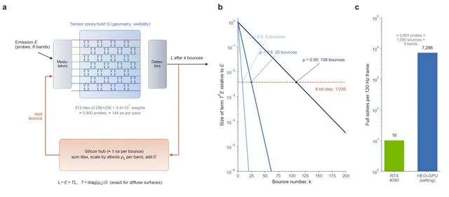
Figure 4. Global illumination on the photonic mesh. a, The bounce loop: emission E enters the core holding the transport matrix, the output is detected, scaled by each band's albedo and re-injected for the next bounce. b, Size of each bounce term relative to the first for average albedos of 0.5, 0.8 and 0.95, against the 8-bit step of 1/256. c, Solves per 120 Hz frame for the RTX 4090 and the HEO-GPU (setting).
8. Size: the area budget at the diffraction limit
An optical waveguide mode cannot be narrower than about λ/(2n), about 0.2 μm in silicon; allowing for coupling and crosstalk, waveguides have to sit a few micrometres apart. A 21st-century thermo-optic MZI is several hundred micrometres long. The setting electro-optic MZI is compressed to about 20 μm × 5 μm, about 10⁴ per square millimetre. The AD102 chip of the RTX 4090 places 76.3 billion transistors on 608.5 mm², about 1.25×10⁸ per mm², about 12,000 times the density of the optical mesh.
The 512 tensor cores hold about 3.4×10⁷ MZI-sized cells and so need about 3,400 mm² of photonic chip, about 5.5 times the area of AD102, or a square about 58 mm on a side. This is the physical reason the HEO-GPU is bigger than today's graphics cards.
9. Temperature: millikelvin precision from the thermo-optic effect
The refractive index of silicon changes with temperature, with a thermo-optic coefficient dn/dT ≈ 1.8×10⁻⁴ K⁻¹. In a waveguide of length L, a temperature change ΔT shifts the phase by:
Eight-bit precision allows a phase error of about 2π/256 ≈ 0.025 rad. If the whole chip warms uniformly, all paths through a mesh have the same length and the phase changes cancel. The danger is a temperature difference between paths:
Table 8. Temperature tolerance (λ = 1550 nm, phase tolerance 0.025 rad)
| Case | Path length L | Phase sensitivity | Allowed temperature difference |
|---|---|---|---|
| Between the arms of one setting MZI | 20 μm | 0.015 rad/K | About 1.7 K |
| Between the arms of a present-day thermo-optic MZI | 200 μm | 0.15 rad/K | About 0.17 K |
| Accumulated along different paths through one mesh | 5.1 mm | 3.7 rad/K | About 7 mK |
| Accumulated through a full tensor core | 10.3 mm | 7.5 rad/K | About 3 mK |
The original concept's claim that "a 0.1 °C difference between left and right ruins everything" holds. A 0.1 K difference across a 5 mm path produces a phase error of about 0.36 rad, 15 times the tolerance; across a full core it is about 30 times. Locking the chip at 25.000 ± 0.001 °C leaves about a threefold margin against the 3 mK limit of a full core. The millikelvin requirement in the film is not an exaggeration; it follows directly from 8-bit precision. Online calibration, with monitor photodiodes correcting the phases every millisecond, can then remove slow drift.
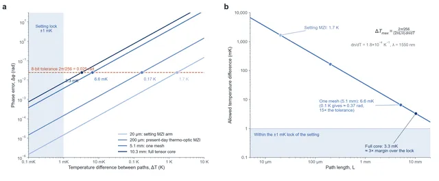
Figure 5. Thermal tolerance. a, Phase error against temperature difference for path lengths of 20 μm, 200 μm, 5.1 mm and 10.3 mm, with the 8-bit tolerance; intersections give the limits in Table 8. b, Allowed temperature difference against path length, with the setting's ±1 mK lock marked.
10. HEO-GPU: what a graphics card of 2400 looks like
Put these parameters into one card and you get the hybrid Heterogeneous Electro-Optical GPU (HEO-GPU) imagined for the film. Each feature of its appearance has a physical reason:
Table 9. HEO-GPU appearance and physical basis
| Part | Appearance | Physical basis |
|---|---|---|
| Overall | Full length and height, four slots, with a support jack; CNC-machined aluminium and carbon-fibre armour | About 3,400 mm² of photonic chip; vibration at the nanometre scale changes optical path lengths |
| Core | Co-packaged electronics and photonics: a silicon hub around a central photonic chip with a glassy sheen | Electronics handles FP32, FP64 and logic; photonics handles 8-bit matrices |
| Light supply | A tunable InP laser module plugged into the tail, 8 colours in the 1550 nm band; an exposed bundle of polarisation-maintaining fibre in orange Kevlar armour | Silicon does not emit light efficiently; the mesh needs coherent light of a single polarisation |
| Cooling | Dual-zone cold plate: a boiling zone carries away about 200 W of electronic heat; a thermoelectric zone holds 25.000 ± 0.001 °C | Thermo-optic effect: temperature differences across a core must stay below 3 mK |
| Connectors | One DisplayPort kept; the main interface is high-density MPO/MTP fibre ports | Rendered output is pumped directly as optical signals into light-field displays |
In effect it is a descendant of the 4090 with a tensor coprocessor made of light added on.
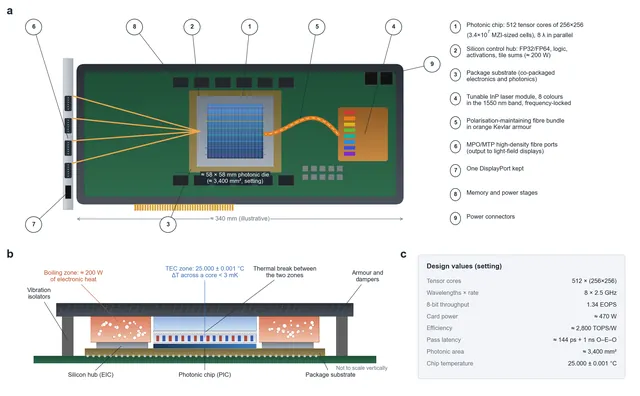
Figure 6. The HEO-GPU (setting). a, Top view with the cooler removed: silicon control hub, central photonic chip of 512 tensor cores, laser module and fibre ports. b, Cross-section through the package and the dual-zone cold plate. c, Design values.
11. Main failure modes
Table 10. Failures and responses
| Failure | Trigger | Consequence | Design response |
|---|---|---|---|
| Thermal drift | Temperature difference across a core > 3 mK | Phase error exceeds the 8-bit tolerance | Dual-zone temperature control and millisecond online calibration |
| Wavelength drift | Laser temperature or ageing | Dispersion increases errors across bands | Frequency-locked lasers; W no more than 8 |
| Optical power noise | Laser intensity fluctuations | Effective precision falls | Normalisation against a reference channel |
| Phase-shifter ageing | Long-term drive | Weight errors | Periodic self-calibration |
| Weight-reload bottleneck | Matrices larger than 3.4×10⁷ weights | Tiling and data movement dominate the time | Keep large matrices resident; suits inference and fixed scenes |
| Conversion bottleneck | Every bounce needs an optical–electrical–optical step | Latency measured in ns rather than ps | Setting: 10 fJ, nanosecond-class converters |
| Vibration | Chassis and fan vibration | Optical path jitter | Damping armour; no air cooling |
From one interferometer to a whole graphics card, every figure of merit in optical computing traces back to a physical law. Latency comes from the speed of light, throughput from N² parallelism, the energy floor from the graininess of photons, the precision ceiling from noise and temperature, and the size from diffraction. The engineers of 2400 turn each of these constraints into a design parameter. What they end up with is a coprocessor that knows what it should do and what it should leave to electronics, rather than a general-purpose "photonic computer".
References and basis of calculation
- M. Reck et al. (1994), Experimental realization of any discrete unitary operator, Physical Review Letters 73: triangular MZI mesh.
- W. R. Clements et al. (2016), Optimal design for universal multiport interferometers, Optica 3: rectangular mesh.
- Y. Shen et al. (2017), Deep learning with coherent nanophotonic circuits, Nature Photonics 11: MZI optical neural network demonstration.
- T. Wang et al. (2022), An optical neural network using less than 1 photon per multiplication, Nature Communications 13: photon number and precision.
- D. A. B. Miller (2017), Attojoule optoelectronics for low-energy information processing and communications, Journal of Lightwave Technology 35: optoelectronic conversion energy.
- J. T. Kajiya (1986), The rendering equation, SIGGRAPH: the rendering equation.
- J. Alman and V. Vassilevska Williams (2021), A refined laser method and faster matrix multiplication: ω < 2.3729; later work has lowered the bound to about 2.371.
- NVIDIA, Ada GPU architecture whitepaper; RTX 4090 and RTX 5090 specifications: FP32 and tensor throughput, power, transistor count. The 5090 FP8 dense value is derived from the official 3,352 AI TOPS (FP4, sparse).
- Basis of calculation: silicon waveguide group index 4.2 and effective index about 2.4; silicon thermo-optic coefficient 1.8×10⁻⁴ K⁻¹; 8-bit phase tolerance 2π/256; shot-noise criterion $n\ge(2^{B})^{2}$; core insertion loss 6 dB, laser wall-plug efficiency 40% and DAC/ADC 10 fJ are setting values; GPU comparison at 8-bit-class dense tensor peak.
Appendix A. Main symbols
Table 11. Symbols
| Symbol | Meaning | Symbol | Meaning |
|---|---|---|---|
| N | Core dimension (matrix side) | $n_g$ | Waveguide group index |
| M | Tensor cores per card | t | Transit time through a core |
| f | Modulation rate | B | Effective precision (bits) |
| W | Number of wavelength channels | n | Photons per output |
| R | Card operation rate | hν | Photon energy |
| U, Σ, V | Factors of the singular value decomposition | T | Light-transport matrix |
| $f_r$ | Bidirectional reflectance distribution function | L, E | Radiance vector / emission vector |
| Δφ | Phase error | dn/dT | Thermo-optic coefficient |