
Terraforming Mars: Air, Magnetic Shields and Orbital Mirrors
The three connected engineering ideas behind Engineering Mars, and the questions a real planetary transformation would need to answer.
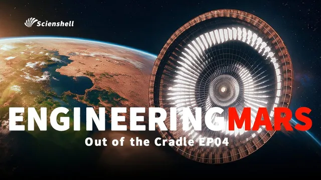
In Engineering Mars, a transformed landscape is the visible result of several much larger projects. Imported material builds an atmosphere and supplies water. A superconducting ring generates a magnetic shield. Two enormous mirrors join direct sunlight to illuminate the surface from three directions.
These are devices in the film’s imagined future. No existing program has established that they could produce its inhabited Mars. Yet the setting invites a serious engineering question: what would have to balance for that landscape to exist?
The answer begins with inventories and operating conditions. A planet needs enough gas of the right composition, an energy balance compatible with its water cycle, and infrastructure that remains controllable as the environment changes. The calculations below are deliberately simple estimates of scale. Their numerical scenarios are assumptions for analysis, not forecasts or certified habitat specifications.
1. Define the environment before designing the machines
“Habitable” is too broad to serve as a system requirement. A greenhouse that reduces the pressure difference across a settlement’s walls, an environment where people use breathing equipment, and an atmosphere supporting ordinary outdoor life are different projects. Their gas inventories, acceptable failure modes and construction sequences would differ substantially.
A design should specify surface pressure at a stated reference elevation; oxygen and carbon-dioxide partial pressures; temperature distributions through a full year; water availability; and limits on dust, toxic contaminants and radiation. An annual average cannot substitute for a winter minimum or a heat wave. The atmosphere must also work across a planet with substantial topography.
For the calculations here, adopt a spherical Mars with radius 3,389.5 km, gravity 3.73 m/s², and incident sunlight 586 W/m² at a representative orbital distance. These are based on NASA’s Mars Fact Sheet. Use 600 Pa as a rounded present-atmosphere reference, rather than a pressure applicable at every place and season. The reference surface area is then:
$$ A = 4\pi R^2 = 1.44 \times 10^{14}\ \mathrm{m^2}. $$
We will compare total pressures of 1, 10 and 100 kPa. The last is an illustrative one-bar benchmark, not a claim that Earth’s pressure is the only possible design choice. None of these pressure values, by itself, establishes breathable air or a warm climate.
2. The atmosphere is a mass budget
Integrating hydrostatic balance gives a useful first estimate for a thin atmosphere on a spherical planet:
$$ M_{\mathrm{atm}} \approx \frac{A p_s}{g}. $$
Here pₛ is representative surface pressure in pascals, A is area in square metres, and g is gravity in metres per second squared. Pressure divided by gravity gives column mass in kg/m². Multiplication by area gives atmospheric mass in kilograms. This approximation neglects topography, vertical changes in gravity and the precise reference surface; it is appropriate for estimating scale, not closing a detailed planetary inventory.
| Reference total pressure | Approximate atmospheric mass |
|---|---|
| 600 Pa, rounded present reference | 2.32 × 10¹⁶ kg |
| 1 kPa | 3.87 × 10¹⁶ kg |
| 10 kPa | 3.87 × 10¹⁷ kg |
| 100 kPa | 3.87 × 10¹⁸ kg |
Raising this reference atmosphere to 100 kPa requires a net additional atmospheric inventory of about 3.85 × 10¹⁸ kg. If it accumulated uniformly over an assumed 1,000 Earth years, the average net addition would be 1.22 × 10⁸ kg/s. That is a scale calculation, not a proposed schedule. Gas consumed by rock reactions, frozen into deposits, dissolved in water or lost to space would increase gross production beyond this net requirement.
The changing inventory can be written as:
$$ \frac{dM_{\mathrm{atm}}}{dt} = \dot M_{\mathrm{release}} + \dot M_{\mathrm{import}}
- \dot M_{\mathrm{sequestration}} - \dot M_{\mathrm{escape}}.
$$
Every term needs a measurement method and an uncertainty range. Releasing gas once is insufficient if the changing climate promptly freezes or chemically binds it elsewhere. Conversely, gas stored in a cap has moved between reservoirs; it has not necessarily escaped the planet.
How much carbon dioxide can Mars supply?
The strongest constraint is the distinction between material that exists and material that can be mobilized. Jakosky and Edwards examined polar deposits, adsorption in the regolith, carbonate minerals and atmospheric loss. Their 2018 inventory study used about 20 mbar, or 2 kPa, as a representative upper pressure obtainable from readily mobilized CO₂ under the evidence and technological constraints they considered. They found no known accessible reservoir sufficient for the proposed planetary warming.
This is not proof that the deep crust contains no additional carbon. It means that unknown carbon cannot be entered into an engineering budget as recoverable feedstock. A deposit requires concentration, depth, extraction yield, process energy and waste estimates. Carbon bound in rock is not a tank of compressed gas waiting for a valve.
The film’s imported asteroids and ice therefore represent a major assumption about its civilization: it can operate a transport and processing economy far beyond present capabilities. That infrastructure is the connection to Solar Express. A delivery program must specify composition as well as tonnage, and explain how material is captured and processed without repeatedly destroying the environment it is intended to build.
For scale, suppose the additional 3.85 × 10¹⁸ kg arrived with an assumed residual speed of 5 km/s relative to the planet. Its kinetic energy would be:
$$ E = \tfrac12 Mv^2 \approx 4.81 \times 10^{25}\ \mathrm{J}. $$
Spread over the same hypothetical millennium, that is 1.52 × 10¹⁵ W of mechanical energy to manage. It is not necessarily all deposited as surface heat: a design could dissipate or redirect energy during capture. The calculation shows why arrival speed, trajectory and energy disposal are first-order requirements rather than incidental logistics.
3. Pressure, breathable air and oxygen are different inventories
A dense CO₂ atmosphere is not breathable. Nor can a warming atmosphere simply be replaced with oxygen without reconsidering climate and fire behaviour. A design needs separate budgets for greenhouse gases, oxygen and a suitable buffer gas, together with their production and removal pathways.
Consider an explicitly hypothetical dry atmosphere containing 21% O₂ and 79% N₂ by mole, at 100 kPa. This is a convenient accounting example, not a complete atmospheric prescription. Its oxygen partial pressure is 21 kPa. To calculate the oxygen mass, however, one must account for molecular mass:
$$ \overline{\mu} = 0.21 \times 32 + 0.79 \times 28 = 28.84\ \mathrm{g\,mol^{-1}}. $$
$$ M_{\mathrm{O_2}} = M_{\mathrm{atm}}\frac{0.21 \times 32}{28.84} \approx 9.02 \times 10^{17}\ \mathrm{kg}. $$
The corresponding nitrogen inventory is 2.97 × 10¹⁸ kg. In a well-mixed atmosphere, species share collisions and pressure support; multiplying each partial pressure independently by A/g would give the wrong species mass. Mole fraction and mass fraction are different quantities.
The nitrogen requirement deserves as much attention as oxygen production. Curiosity’s SAM measurements provide evidence for nitrogen-bearing material interpreted as nitrates in sampled sediments. Stern and colleagues’ results are evidence of a local resource and past chemistry, not a demonstrated recoverable inventory for an entire atmosphere. Selecting nitrogen as a buffer does not establish that Mars can supply the amount required.
Oxygen also needs a complete chemical balance. If the illustrative oxygen inventory came entirely from water electrolysis, the reaction would be:
$$ 2\,\mathrm{H_2O} \rightarrow 2\,\mathrm{H_2} + \mathrm{O_2}. $$
This would require at least 1.01 × 10¹⁸ kg of water feed and produce 1.13 × 10¹⁷ kg of hydrogen, before process losses. The hydrogen needs a destination. Letting it recombine with oxygen reverses the desired storage; retaining or exporting it creates another industrial stream. Producing oxygen from CO₂ instead leaves carbon monoxide or a further processed carbon product that must also be managed.
There is a real experimental foundation for local oxygen production. NASA’s MOXIE experiment extracted oxygen from Martian CO₂, producing 122 grams over its mission and reaching 12 grams per hour. Its value is demonstrating chemistry, purity and operation under Martian conditions. It does not demonstrate the factories, power supply or maintenance system needed for the 2.86 × 10⁷ kg/s of oxygen accumulation implied by our deliberately enormous millennium scenario.
Biology would not remove these balances. Photosynthetic oxygen accumulates only to the extent that its reducing products avoid recombination. Respiration, decomposition and reactions with reduced minerals consume oxygen. Any biological stage therefore needs measured net productivity and sinks, rather than a landscape’s apparent greenness as proof of atmospheric progress.
4. Close the thermal balance
With solar flux S and an assumed Bond albedo α = 0.25, a simple globally averaged absorbed flux is:
$$ F_{\mathrm{abs}} = \frac{(1-\alpha)S}{4} \approx 110\ \mathrm{W\,m^{-2}}. $$
The factor of four compares the sunlight intercepted by a disk with the area of a sphere. In radiative equilibrium:
$$ \sigma T_{\mathrm{eff}}^4 = F_{\mathrm{abs}}, \qquad T_{\mathrm{eff}} \approx 210\ \mathrm{K}. $$
A blackbody at 273 K would emit about 315 W/m².
Those numbers do not mean that every square metre of Mars needs another 205 watts of sunlight to obtain liquid water. Effective emission temperature describes radiation escaping to space; it is not necessarily surface temperature. Atmospheric absorption, convection, clouds and infrared emission determine the relationship. A greenhouse changes where radiation escapes, while water and ice alter albedo, latent heat and circulation.
Forget and colleagues’ three-dimensional early-Mars simulations illustrate the difficulty: more CO₂ does not translate into unlimited warming, and condensation can remove gas from the atmosphere. Their simulations concern an earlier, fainter Sun and cannot be copied directly into a future-Mars forecast. They establish why composition, clouds, topography and circulation belong inside the model rather than being appended to a temperature estimate.
A future design would need ensembles of coupled climate, photochemistry and surface-reservoir simulations. It should track seasonal liquid water and precipitation, not merely crossing a global average of 273 K. It must also calculate how much greenhouse gas could remain in a later breathable atmosphere. A CO₂-rich construction phase and a low-CO₂ inhabited phase do not automatically share the same thermal solution.
5. Orbital mirrors: collecting power is only the beginning
Orbital reflectors have a history in terraforming proposals. Zubrin and McKay’s 1993 paper discussed a mirror of roughly 125 km radius for polar heating. That was a proposed intervention with particular assumptions, not a demonstrated route to global habitability. The film’s two additional “suns” make redirected sunlight visible as part of daily life; their appearance does not specify their engineering capacity.
Consider a separate design exercise: deliver an extra 20 W/m² of globally averaged absorbed power. This is a chosen test target, not a calculated warming requirement. It corresponds to:
$$ P_{\mathrm{abs}} = A\Delta F \approx 2.89 \times 10^{15}\ \mathrm{W}. $$
Assume mirror reflectivity ρ = 0.90 and net utilization η = 0.50. Here utilization includes projected area, interception by Mars, eclipse and operating duty, and the fraction of delivered light ultimately absorbed by the planet. Under these assumptions, physical mirror area must be:
$$ A_m = \frac{A\Delta F}{S\rho\eta} \approx 1.09 \times 10^{13}\ \mathrm{m^2}. $$
That is about 10.9 million km².
A circular mirror of 100 km radius would provide about 8.28 × 10¹² W of absorbed power under the same accounting, equivalent to only 0.057 W/m² averaged over Mars. Approximately 350 such mirrors would meet the chosen 20 W/m² target. This comparison concerns global power; a smaller reflector could still have a substantial local effect. It also shows why two bright points in the sky cannot establish a planetary energy budget.
At an assumed membrane loading of 10 g/m², the calculated total area represents 1.09 × 10¹¹ kg of reflecting sheet alone. Booms, wiring, actuators, navigation equipment, repair systems and reserves would add mass. Manufacturing area, deployment yield and replacement rate would matter alongside launch capacity.
Orbit and attitude are part of the optical system
A reflector must orient its normal approximately along the bisector of incoming and outgoing light directions. Tilting reduces collected power and changes radiation-pressure forces. Orbit selection must accommodate eclipses, changing Sun–Mars geometry, local illumination schedules and collision avoidance. A freely orbiting mirror does not remain above a selected town; a continuously displaced configuration needs a demonstrated force and navigation balance.
The force from sunlight is small per square metre but persistent. For an ideal normally illuminated perfect reflector:
$$ p_{\mathrm{rad}} = \frac{2S}{c} \approx 3.91 \times 10^{-6}\ \mathrm{Pa}. $$
That is about 3.91 micropascals (µPa) at the chosen solar flux. NASA-supported solar-sail research derives the associated force and torque. Dividing by the hypothetical 10 g/m² loading gives an ideal sheet acceleration of 3.91 × 10⁻⁴ m/s²—about 34 m/s of velocity change in one Earth day if its direction remained fixed. This is an illustrative force scale, not a station-keeping prediction for the heavier, tilted assembly.
Pointing must also account for the Sun’s finite angular extent, membrane shape, segment errors and the target’s motion. A mirror cannot be treated as an arbitrary point source. Loss of attitude knowledge should send reflected light away from inhabited targets, with independent limits on allowed ground irradiance and exposure duration.
Longevity requires separate optical and structural tests. NASA laboratory work on candidate sail films found that radiation exposure could damage mechanical properties and a reflective layer without a corresponding significant change in the measured solar absorptance or thermal emittance of that specimen. A mirror can therefore remain optically useful while becoming structurally vulnerable. A credible lifetime budget needs measured degradation under the intended orbit’s environment, plus inspection, isolation and replacement plans.
6. What would a magnetic shield actually protect?
MAVEN’s atmospheric measurements support substantial historical atmospheric loss to space. That gives retention a legitimate place in the film’s systems architecture. It does not mean an unmagnetized atmosphere disappears immediately, nor does it supply a future escape rate for an artificially thickened atmosphere.
Real concepts differ from the film’s superconducting ring. A NASA conference abstract by Green and colleagues explored an artificial dipole near Mars–Sun L1. Bamford and colleagues examined other configurations, including a current-carrying particle ring. These are research concepts with major unresolved engineering requirements, not validated planetary protection systems.
A simplified pressure balance illustrates one scale:
$$ \frac{B^2}{2\mu_0} \approx P_{\mathrm{sw}}, \qquad B \approx \sqrt{2\mu_0P_{\mathrm{sw}}}. $$
For an assumed solar-wind pressure of 1 nPa, this gives B ≈ 50 nT. Here μ₀ is the permeability of free space. This is a local field at an idealized plasma boundary. It does not specify generator field, coil current, conductor mass, standoff distance or power. Those require geometry and plasma dynamics; a superconducting conductor also needs cryogenic operation, support against electromagnetic forces and a safe response to a quench.
The success measure should be reduced integrated atmospheric loss under a range of solar conditions, not simply a visible magnetosphere. Gunell and colleagues’ escape modelling shows why: magnetic geometry can suppress some escape mechanisms while opening others through polar caps and cusps. Thermal and photochemical escape require their own treatment. Atmospheric chemistry, upper-atmosphere heating and gas supply remain part of the retention problem.
Radiation protection is a related but separate requirement. Our 100 kPa atmosphere has a column mass of about 26,800 kg/m², compared with 161 kg/m² at the 600 Pa reference. That additional material changes particle transport even without a magnetic shield. Predicting dose still requires composition-dependent radiation calculations, including secondary particles; a field strength or a pressure reading cannot substitute for them.
The engineering trade should therefore compare additional atmospheric supply, shielding infrastructure and continued protected habitats against a specified retention horizon and radiation target. A shield cannot create missing nitrogen or oxygen. Higher pressure cannot eliminate the need to understand escape. Neither should be declared a prerequisite for the other without a quantitative comparison.
7. A demonstration program with measurable exits
The credible first step is a sequence of experiments that can invalidate assumptions cheaply, while settlements remain independently habitable.
Resource and chemistry phase. Combine orbital surveys, drilling and pilot extraction to estimate recoverable gas inventories with uncertainty bounds. Measure energy per kilogram, contaminants, waste and oxygen uptake by representative soils. Proceed only when the conservative recoverable inventory closes the chosen stage’s budget, including sinks and reserves. A detection without an extraction and mass balance is insufficient.
Contained environment phase. Operate instrumented test enclosures through seasonal cycles. Track every imported, produced, stored and lost gas stream, while measuring water, dust and surface chemistry. A proposed program might require mass-balance closure within 5% of throughput before increasing scale; this is an illustrative acceptance criterion, not an existing standard. Persistent unexplained losses should stop expansion.
Orbital control phase. Fly a small reflector with independent ground radiometry, navigation and shape measurements. Demonstrate delivered power, seasonal pointing, degradation and deliberate safe-mode transitions. An illustrative test goal would be predicted versus measured absorbed power within 10%, with irradiance limits set separately for the actual target. Test a relevant magnetic configuration through measured particle distributions and escape fluxes, comparing conditions against a defensible unperturbed baseline.
Coupled-system phase. Feed these results into climate and escape models, publish uncertainty ranges, and test whether pressure, composition and seasonal water targets can coexist. Examine prolonged mirror outages, shield failures and interrupted supply before committing to planetary changes. Any transition must leave inhabitants with independent pressure, breathing gas and shelter for the credible recovery interval.
No demonstrator would authorize a simple leap to planetary scale. Each resolves a particular question: whether a reservoir is recoverable, a process produces a net surplus, a reflector remains controllable, or a shield reduces the relevant loss. Unknowns should remain visible in the design until measurements replace them.
The lasting image in Engineering Mars is a world whose inhabitants encounter infrastructure as weather, light and landscape. Reaching that setting would require a civilization to close all of these balances together, and keep closing them for generations. The film supplies the destination. Engineering begins with specifying what must be measured on the way.
Watch Engineering Mars free, or explore Out of the Cradle for the imagined power, transport and settlements surrounding this future Mars.
Sources and further reading
- NASA: Mars Fact Sheet — physical and atmospheric reference values.
- Jakosky and Edwards (2018): Inventory of CO₂ available for terraforming Mars — assessed carbon reservoirs and mobilization limits.
- Stern et al. (2015): Evidence for indigenous nitrogen in sedimentary and aeolian deposits — Curiosity SAM measurements.
- NASA/JPL (2023): MOXIE completes its Mars mission — demonstrated oxygen production.
- Forget et al. (2013): Three-dimensional modelling of the early Martian climate — CO₂ climate and condensation simulations under an early Sun.
- Zubrin and McKay (1993): Technological requirements for terraforming Mars — historical engineering proposals, including polar reflectors.
- Swartzlander (2018): Steering of solar sails using optical lift force — radiation-pressure force and torque analysis.
- Kang et al. (2017): Simulated space-environment effects on a candidate solar-sail material — membrane degradation testing.
- NASA (2017): MAVEN reveals atmospheric loss — mission results on atmospheric history.
- Green et al. (2017): A future Mars environment for science and exploration — exploratory L1 magnetic-dipole concept.
- Bamford et al. (2022): How to create an artificial magnetosphere for Mars — engineering comparisons between speculative configurations.
- Gunell et al. (2018): Why an intrinsic magnetic field does not protect a planet against atmospheric escape — competing atmospheric-escape pathways.